
Grade Expectations: Exploring A/B Testing & Feature Selection Through Student GPAs

Abstract
I’ve been seeing a lot of demand for A/B testing experience in jobs I’ve been applying to lately. While I’ve done this type of work in academia, I can’t say I’ve formally performed it in a professional context. Not often, but on some occasions when I tell this to recruiters, I can feel the burgeoning hesitation they feel in advancing me to the next step. I’m kind of amazed when this is the limiting factor that prohibits me from advancing, because A/B testing in practice is not actually very complicated. Sure, there may be some more nuance to the context around it in a professional setting that one needs to understand, but the mechanics of the technique itself are not complex. In this post, I’m going to describe exactly what A/B testing is, how to perform it, its use as a feature selection method, and springboard into more advanced feature selection methods. After I’ve given a generalist approach to defining the A/B test, I will implement it in an example around synthetic student GPA data to better showcase its use.
What is A/B testing?
Contrary to the reductionist language I’m seeing online and in interviews, an A/B test is not actually a specific statistical test, but actually a type of experimental design where we sample from a population and split them into a control group and experimental group (groups A and B). Then we subject some type of update from the status-quo to the experimental group and measure the occurrence of some metric between the two groups. Whether you know it or not, you’re probably familiar with some.
Do you understand how in drug trials one group is given a placebo and another group is given some new drug to determine if it has any efficacy? This is an A/B test. Another type of A/B test that I’m being asked if I have experience with is product A/B testing. Let’s take a generic social media company for example. They have a vested interest in increasing the amount of time their users actually use their platform. They have some theory that the layout of their mobile application on a very specific phone is not optimized, thereby losing user engagement on that phone. To test if they can increase user engagement among users of this phone, they might run an A/B test featuring some new layout.
This is the high-level organization of the experimental design: having two groups (A/B) and then impacting a change you’re trying to research the efficacy of one of said groups.
Important Preliminary Details
Before launching an A/B test, it’s essential to ensure several foundational conditions are met. These safeguards help ensure that the results are valid, interpretable, and actionable.
An appropriate sample size
Before you run an A/B test, it’s important to make sure your sample size is large enough. If your sample is too small, you might not be able to tell whether the difference you see between groups is real or just due to random chance.
Let’s take a coin flip as an example. If I flipped a quarter 3 times and got heads twice, I might think heads comes up more often than tails. But with such a small number of flips, that result could easily be a fluke. Now imagine I flipped the coin 1,000 times and got 520 heads — I’d feel much more confident saying the coin is probably fair (or close to it).
A/B tests work the same way. The more people or events included in the test, the more confident we can be in the results. In fact, the statistical test we use will output a number — often called a p-value or confidence level — that tells us how likely it is that the difference between groups is real. This number is heavily influenced by how much data we collect.
That’s why planning for sample size is so important. If we want to be very confident in our results, we’ll need a large enough sample. But in real-world settings, there’s often a trade-off: running a longer test gives us more certainty, while shorter tests might give faster answers (and quicker product changes) but with more uncertainty.
Reasonably identical features along A/B
For an A/B test to be fair, the control group and the experiment group should be similar in every important way except for the thing you’re testing.
Imagine testing a new medication designed to help people with a specific illness. It wouldn’t make sense to include people without that illness in the experiment group but only people with the illness in the control group. That would make it impossible to know if differences in results were due to the medicine or just differences in who was in each group.
Similarly, if there’s another health condition that could affect how well the medicine works, you’d want to make sure that condition is either equally represented in both groups or excluded altogether. If not, the results could be misleading.
This idea applies to any A/B test: the groups should be as similar as possible so you can be confident that differences in outcomes are caused by the change you made — not other factors.
Random Sampling
To make sure the control and experiment groups are as similar as possible, we assign users to each group using random sampling.
Random sampling means each user has an equal chance of being placed in either group. This helps avoid bias — so the groups don’t differ in any unexpected ways that could affect the results.
By randomly assigning users, we can be more confident that any differences we see are due to the change we’re testing, not other factors.
So if A/B is an experimental design, what’s the test?
So, we’ve organized equal-sized and similar-featured group A and B to run a test… now what? Well, that all depends on what we’re trying to measure here. Are we expecting a higher frequency of a binary outcome (a patient is cured / not cured), or higher rates of a continuous value (the changes to a study app helped yield higher SAT scores among users)? Does our continuous value follow an approximately normal distribution? All these help us to choose the type of test we will run.
The Student’s T-Test
A very common type of statistical test run in an A/B experiment design is the Student’s T-test (published by a statistician and brewery chemist using the pseudonym student). This is used to compare the mean value of a variable of interest across our groups to determine if there is a statistically significant difference. I.e., is the average weight between this group that took a new weight loss pill and their placebo control group different and is that difference meaningful or just random chance? Note that this is not the same question as does this drug cause weight loss? A/B tests do NOT imply causality.
There are a few different types of t-test depending (one sample, two sample, paired), but without going into these I’ll just say two sample tests are what are used in A/B testing (two groups = two samples).
Z-test
Similar to the Student’s T-Test, however this measures difference in a binary value. I.e., does this product change yield more customer sign-ups than the status-quo. This has similar one sample, two sample, paired flavors as the t-test.
Other Tests
These are the two primary tests that get utilized in A/B testing. There are a myriad of other statistical tests that fit different purposes in particular scenarios. Non-parametric counterparts to the t and z-test (Mann-Whitney U and Chi-square tests, respectively) can be used in lieu of the t and z-test when the assumption of normality is not met. However they compare sample medians or ranks, where as the t and z-test compare means or proportions.
There are also tests that extend beyond the A/B structure. ANOVA (analysis of variance) can be used to detect if there is some statistically significant variance among any number of groups, not just two.
In Practice
That was a bit more of a foreword than I probably wanted, but there was some exposition I needed to do for those unfamiliar. Now, I want to jump into a set of data I came across to show how we can use the common tests used in A/B experiment design for feature selection.
So, here we have a synthetic dataset representing the exam scores of 80,000 students and potentially related predicting variables.
This is a head of all the data to familiarize yourself with the features.
And some descriptive summary statistics to understand the shape of the data a bit more.
Data Frame Summary
grades_and_features
Dimensions: 80000 x 31Duplicates: 0
| Variable | Stats / Values | Freqs (% of Valid) | Graph | Missing | ||||||||||||||||||||||||||||||||||||||||||||||||||||||||||||||||
|---|---|---|---|---|---|---|---|---|---|---|---|---|---|---|---|---|---|---|---|---|---|---|---|---|---|---|---|---|---|---|---|---|---|---|---|---|---|---|---|---|---|---|---|---|---|---|---|---|---|---|---|---|---|---|---|---|---|---|---|---|---|---|---|---|---|---|---|---|
| student_id [numeric] |
|
80000 distinct values |  |
0 (0.0%) | ||||||||||||||||||||||||||||||||||||||||||||||||||||||||||||||||
| age [numeric] |
|
13 distinct values |  |
0 (0.0%) | ||||||||||||||||||||||||||||||||||||||||||||||||||||||||||||||||
| gender [character] |
|
|
 |
0 (0.0%) | ||||||||||||||||||||||||||||||||||||||||||||||||||||||||||||||||
| major [character] |
|
|
 |
0 (0.0%) | ||||||||||||||||||||||||||||||||||||||||||||||||||||||||||||||||
| study_hours_per_day [numeric] |
|
13364 distinct values |  |
0 (0.0%) | ||||||||||||||||||||||||||||||||||||||||||||||||||||||||||||||||
| social_media_hours [numeric] |
|
51 distinct values |  |
0 (0.0%) | ||||||||||||||||||||||||||||||||||||||||||||||||||||||||||||||||
| netflix_hours [numeric] |
|
41 distinct values |  |
0 (0.0%) | ||||||||||||||||||||||||||||||||||||||||||||||||||||||||||||||||
| part_time_job [character] |
|
|
 |
0 (0.0%) | ||||||||||||||||||||||||||||||||||||||||||||||||||||||||||||||||
| attendance_percentage [numeric] |
|
601 distinct values |  |
0 (0.0%) | ||||||||||||||||||||||||||||||||||||||||||||||||||||||||||||||||
| sleep_hours [numeric] |
|
81 distinct values |  |
0 (0.0%) | ||||||||||||||||||||||||||||||||||||||||||||||||||||||||||||||||
| diet_quality [character] |
|
|
 |
0 (0.0%) | ||||||||||||||||||||||||||||||||||||||||||||||||||||||||||||||||
| exercise_frequency [numeric] |
|
|
 |
0 (0.0%) | ||||||||||||||||||||||||||||||||||||||||||||||||||||||||||||||||
| parental_education_level [character] |
|
|
 |
0 (0.0%) | ||||||||||||||||||||||||||||||||||||||||||||||||||||||||||||||||
| internet_quality [character] |
|
|
 |
0 (0.0%) | ||||||||||||||||||||||||||||||||||||||||||||||||||||||||||||||||
| mental_health_rating [numeric] |
|
91 distinct values |  |
0 (0.0%) | ||||||||||||||||||||||||||||||||||||||||||||||||||||||||||||||||
| extracurricular_participation [character] |
|
|
 |
0 (0.0%) | ||||||||||||||||||||||||||||||||||||||||||||||||||||||||||||||||
| previous_gpa [numeric] |
|
220 distinct values |  |
0 (0.0%) | ||||||||||||||||||||||||||||||||||||||||||||||||||||||||||||||||
| semester [numeric] |
|
|
 |
0 (0.0%) | ||||||||||||||||||||||||||||||||||||||||||||||||||||||||||||||||
| stress_level [numeric] |
|
91 distinct values |  |
0 (0.0%) | ||||||||||||||||||||||||||||||||||||||||||||||||||||||||||||||||
| dropout_risk [character] |
|
|
 |
0 (0.0%) | ||||||||||||||||||||||||||||||||||||||||||||||||||||||||||||||||
| social_activity [numeric] |
|
|
 |
0 (0.0%) | ||||||||||||||||||||||||||||||||||||||||||||||||||||||||||||||||
| screen_time [numeric] |
|
198 distinct values |  |
0 (0.0%) | ||||||||||||||||||||||||||||||||||||||||||||||||||||||||||||||||
| study_environment [character] |
|
|
|
0 (0.0%) | ||||||||||||||||||||||||||||||||||||||||||||||||||||||||||||||||
| access_to_tutoring [character] |
|
|
|
0 (0.0%) | ||||||||||||||||||||||||||||||||||||||||||||||||||||||||||||||||
| family_income_range [character] |
|
|
|
0 (0.0%) | ||||||||||||||||||||||||||||||||||||||||||||||||||||||||||||||||
| parental_support_level [numeric] |
|
|
 |
0 (0.0%) | ||||||||||||||||||||||||||||||||||||||||||||||||||||||||||||||||
| motivation_level [numeric] |
|
|
 |
0 (0.0%) | ||||||||||||||||||||||||||||||||||||||||||||||||||||||||||||||||
| exam_anxiety_score [numeric] |
|
|
 |
0 (0.0%) | ||||||||||||||||||||||||||||||||||||||||||||||||||||||||||||||||
| learning_style [character] |
|
|
 |
0 (0.0%) | ||||||||||||||||||||||||||||||||||||||||||||||||||||||||||||||||
| time_management_score [numeric] |
|
91 distinct values |  |
0 (0.0%) | ||||||||||||||||||||||||||||||||||||||||||||||||||||||||||||||||
| exam_score [numeric] |
|
65 distinct values |  |
0 (0.0%) |
Generated by summarytools 1.1.4 (R version 4.5.1)
2025-08-27
It’s important to remember, this is synthetic data. Whoever made this has done very well to ensure there are near even distributions between our categorical variables and continuous numeric variables are roughly normally distributed.
Forming a Hypothesis
All inferential statistical tests begin with a hypothesis. For an A/B test we hope or hypothesize that there will be some measurable difference in outcome between two groups.
So let me throw out some arbitrary hypothesis.
The Mechanics of the Test
Assuming you know how to calculate an average and a standard deviation, this is the formula to get the t-statistic that will allow us to compare the means of our two groups.
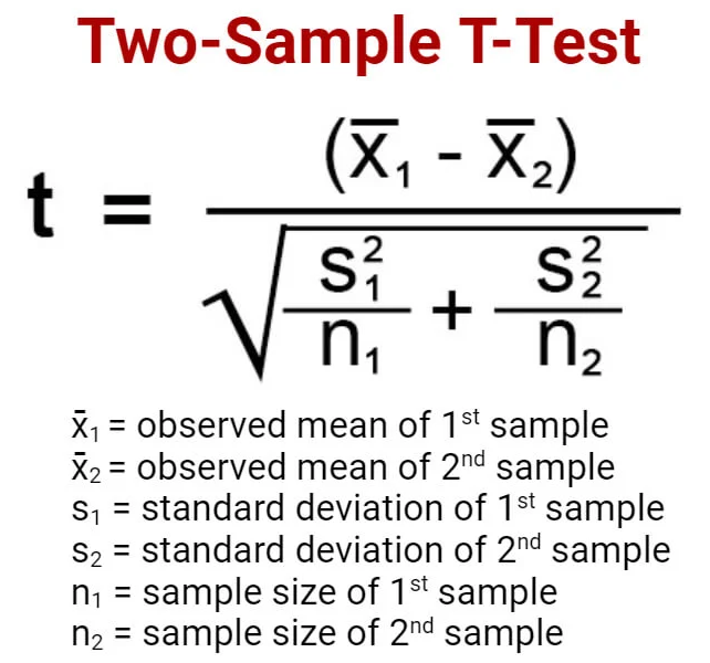
With the value t we do further work to compare against a critical value we obtain from a t-distribution, but going into that is a little further than I want to write about. Just let it be known we can calculate this by hand given some resources - or we can use statistical packages in R to quickly output the results.
# seed for reproducability
set.seed(6391)

# work has been done separately to ensure there are no confounding variables

# sampling 5000 rows of women
rando_women <- grades_and_features %>%
  filter(gender == 'Female') %>%
  .[sample(nrow(.), 5000), ] %>%
  pull(exam_score)

# sampling 5000 rows of men
rando_men <- grades_and_features %>%
  filter(gender == 'Male') %>%
  .[sample(nrow(.), 5000), ] %>%
  pull(exam_score)

t.test(rando_men, rando_women)
##
## Welch Two Sample t-test
##
## data: rando_men and rando_women
## t = 0.25821, df = 9998, p-value = 0.7962
## alternative hypothesis: true difference in means is not equal to 0
## 95 percent confidence interval:
## -0.3994445 0.5206445
## sample estimates:
## mean of x mean of y
## 89.0694 89.0088The p-value tells us how likely it is that the difference in means we observed could happen just by chance if there were no real difference in the population. A p-value of 0.7962 means the observed difference is not statistically significant. Likewise, we can take a look at the means of both groups and see how they are nearly identical. In this case we do not have enough evidence to reject the null hypothesis and must accept that women and men have roughly the same exam scores.
As a Tool for Feature Selection.
Now consider beyond testing various groups for meaningful differences in exam scores, that I was even going so far as to develop to formula to help predict exam score. I could make a linear regression model, or some derivation of this model type, but then how would I go about choosing what features make the most sense? We’ve already seen there’s no meaningful difference in exam scores based on gender. I guess I could just continue applying some inferential test along all the categorical variables in my data, but that could take a long time and would not help me choose amongst the numeric variables.
Advanced Feature Selection Methods
As a little addendum to this primer on inferential methods, I’ll talk a bit about feature selection too. Consider that I want to build a type of model that takes some input and outputs a prediction of exam score. How will I find out what are the most important input variab